Figure组成🔗

Matplotlib是一个Python的绘图库，它在Figure上绘制图像，每个Figure可以包含多个Axes，每个Axes可以理解为一幅图。

Figure🔗

Figure是整个图形的容器，一般使用下面函数之一创建一个Figure：

fig = plt.figure()             # an empty figure with no Axes
fig, ax = plt.subplots()       # a figure with a single Axes
fig, axs = plt.subplots(2, 2)  # a figure with a 2x2 grid of Axes
# a figure with one Axes on the left, and two on the right:
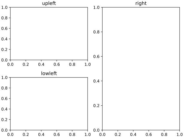
fig, axs = plt.subplot_mosaic([['left', 'right_top'],
                               ['left', 'right_bottom']])

Axes🔗

Axes是一个具有数据空间的图像区域，每个Axes都有一个标题（set_title()）、一个x轴标签（set_xlabel()）和一个y轴标签（set_ylabel()）。Axes是绘图的主要部分。

Axis🔗

Axis设置刻度和限制，并有刻度和刻度标签，刻度位置由Locator确定，刻度标签由Formatter确定。

Artist🔗

在Figure上绘制的所有对象都是Artist，Artist包括Axes、Axis、Line2D等。

绘图函数输入🔗

绘图函数的输入一般来讲是numpy.array或numpy.ma.masked_array，或是其他可以传递给numpy.array的对象。若是像numpy.matrix和pandas的数据对象一般需要先转换为numpy.array：

b = np.matrix([[1, 2], [3, 4]])
b_asarray = np.asarray(b)

大多数方法还能解析可字符串索引的对象，例如dict，structured numpy array或pandas.DataFrame，提供数据的索引作为x和y参数：

np.random.seed(19680801)  # seed the random number generator.
data = {'a': np.arange(50),
        'c': np.random.randint(0, 50, 50),
        'd': np.random.randn(50)}
data['b'] = data['a'] + 10 * np.random.randn(50)
data['d'] = np.abs(data['d']) * 100

fig, ax = plt.subplots(figsize=(5, 2.7), layout='constrained')
ax.scatter('a', 'b', c='c', s='d', data=data)
ax.set_xlabel('entry a')
ax.set_ylabel('entry b')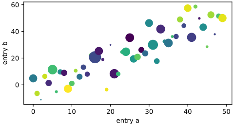

上面代码先创建了一个叫data的dict，装了a，b，c，d四个数组，然后使用scatter函数绘制散点图，x和y参数分别是a和b，color参数是c，size参数是d。

代码风格🔗

显示接口和隐示接口🔗

有两种使用Matplotlib的方法，一种是显式创建Figures和Axes，然后调用它们的方法（OO风格），例如ax.plot(x, y)，另一种是使用pyplot的隐式接口，例如plt.plot(x, y)，这种方法会自动创建Figures和Axes，然后调用它们的方法（pyplot风格）。

第一种如下：

x = np.linspace(0, 2, 100)  # Sample data.

# Note that even in the OO-style, we use `.pyplot.figure` to create the Figure.
fig, ax = plt.subplots(figsize=(5, 2.7), layout='constrained')
ax.plot(x, x, label='linear')  # Plot some data on the Axes.
ax.plot(x, x**2, label='quadratic')  # Plot more data on the Axes...
ax.plot(x, x**3, label='cubic')  # ... and some more.
ax.set_xlabel('x label')  # Add an x-label to the Axes.
ax.set_ylabel('y label')  # Add a y-label to the Axes.
ax.set_title("Simple Plot")  # Add a title to the Axes.
ax.legend()  # Add a legend.

第二种如下：

x = np.linspace(0, 2, 100)  # Sample data.

plt.figure(figsize=(5, 2.7), layout='constrained')
plt.plot(x, x, label='linear')  # Plot some data on the (implicit) Axes.
plt.plot(x, x**2, label='quadratic')  # etc.
plt.plot(x, x**3, label='cubic')
plt.xlabel('x label')
plt.ylabel('y label')
plt.title("Simple Plot")
plt.legend()

另外还有第三种方法，用于将Matplotlib嵌入GUI应用程序中，但这种方法不常用。

一般来说，在复杂的项目中建议使用OO风格，而在需要快速交互工作时，pyplot风格会很方便。

创建辅助函数🔗

可以写函数来简化我们的操作：

def my_plotter(ax, data1, data2, param_dict):
    """
    A helper function to make a graph.
    """
    out = ax.plot(data1, data2, **param_dict)
    return out

data1, data2, data3, data4 = np.random.randn(4, 100)  # make 4 random data sets
fig, (ax1, ax2) = plt.subplots(1, 2, figsize=(5, 2.7))
my_plotter(ax1, data1, data2, {'marker': 'x'})
my_plotter(ax2, data3, data4, {'marker': 'o'})

这里定义了一个函数my_plotter，然后绘制了两个图。

Artists风格🔗

对于Artists的样式选择，可以在绘图时指定，也可以在绘图使用setter指定：

fig, ax = plt.subplots(figsize=(5, 2.7))
x = np.arange(len(data1))
ax.plot(x, np.cumsum(data1), color='blue', linewidth=3, linestyle='--')
l, = ax.plot(x, np.cumsum(data2), color='orange', linewidth=2)
l.set_linestyle(':')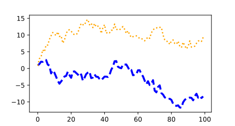

这里第一条线在绘图时指定了linestyle，第二条线在绘图后使用set_linestyle指定了linestyle。

颜色🔗

对于颜色的定义，参照Specifying colors，对于一个scatter，标记边缘和内部可以是不同颜色：

fig, ax = plt.subplots(figsize=(5, 2.7))
ax.scatter(data1, data2, s=50, facecolor='C0', edgecolor='k')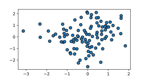

线宽、线型和标记大小🔗

线宽一般是以点为单位，用于有线条的Artists，线型的定义参照Linestyles。

标记的大小取决于绘图的方法，plot大小是一个点，scatter大小与可视区域成比例。标记的样式定义可以参照matplotlib.markers：

fig, ax = plt.subplots(figsize=(5, 2.7))
ax.plot(data1, 'o', label='data1')
ax.plot(data2, 'd', label='data2')
ax.plot(data3, 'v', label='data3')
ax.plot(data4, 's', label='data4')
ax.legend()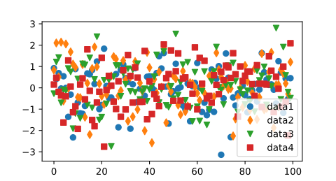

标签🔗

Axes标签和文本🔗

用set_xlabel、set_ylabel和set_title在指定位置添加文本，也可以用text添加文本到绘图中（详细见Text in Matplotlib）：

mu, sigma = 115, 15
x = mu + sigma * np.random.randn(10000)
fig, ax = plt.subplots(figsize=(5, 2.7), layout='constrained')
# the histogram of the data
n, bins, patches = ax.hist(x, 50, density=True, facecolor='C0', alpha=0.75)

ax.set_xlabel('Length [cm]')
ax.set_ylabel('Probability')
ax.set_title('Aardvark lengths\n (not really)')
ax.text(75, .025, r'$\mu=115,\ \sigma=15$')
ax.axis([55, 175, 0, 0.03])
ax.grid(True)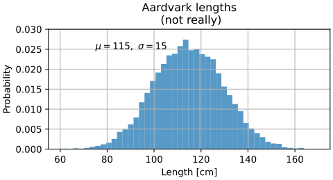

所有函数text方法都会返回一个matplotlib.text.Text实例，可以通过传入参数来改变文本样式（详细见Text properties and layout）：

t = ax.set_xlabel('my data', fontsize=14, color='red')

在文本中使用数学表达式🔗

Matplotlib支持TeX数学表达式，使用$来表示数学表达式：

ax.set_title(r'$\sigma_i=15$')

这里的r前缀表示里面内容是原始字符串而不是将反斜杠视为Python转义。Matplotlib内置有TeX表达式解析器和输出引擎，另外也可以使用LaTeX来进行文本渲染（详细见Text rendering with LaTeX）。

附注🔗

注释某个点，通常是用箭头指向该点，然后连接到一处文本：

fig, ax = plt.subplots(figsize=(5, 2.7))

t = np.arange(0.0, 5.0, 0.01)
s = np.cos(2 * np.pi * t)
line, = ax.plot(t, s, lw=2)

ax.annotate('local max', xy=(2, 1), xytext=(3, 1.5),
            arrowprops=dict(facecolor='black', shrink=0.05))

ax.set_ylim(-2, 2)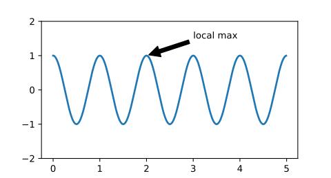

这个实例，使用annotate方法添加了一个指向(2, 1)的箭头，箭头连接到(3, 1.5)。

图例🔗

一般我们使用legend方法来添加图例（详细见Legend guide）：

fig, ax = plt.subplots(figsize=(5, 2.7))
ax.plot(np.arange(len(data1)), data1, label='data1')
ax.plot(np.arange(len(data2)), data2, label='data2')
ax.plot(np.arange(len(data3)), data3, 'd', label='data3')
ax.legend()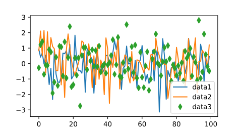

Axis刻度🔗

每个Axes都有两个或三个Axis对象，这些参数控制Axis的缩放、刻度定位和刻度格式。

Scales🔗

除了线性刻度，Matplotlib还提供了非线性刻度（例如对数刻度），有loglog、semilogx、semilogy等众多方法（详见Scales overview）。这里我们手动设置：

fig, axs = plt.subplots(1, 2, figsize=(5, 2.7), layout='constrained')
xdata = np.arange(len(data1))  # make an ordinal for this
data = 10**data1
axs[0].plot(xdata, data)

axs[1].set_yscale('log')
axs[1].plot(xdata, data)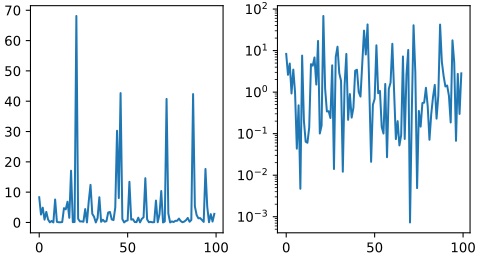

这里将第二幅图的y轴设置为对数刻度。

Tick🔗

每个Axis都有一个刻度定位和格式化工具用于选择刻度线和标签，这里一个简单的接口是set_xticks和set_yticks（详细见Tick locators和Tick formatters）：

fig, axs = plt.subplots(2, 1, layout='constrained')
axs[0].plot(xdata, data1)
axs[0].set_title('Automatic ticks')

axs[1].plot(xdata, data1)
axs[1].set_xticks(np.arange(0, 100, 30), ['zero', '30', 'sixty', '90'])
axs[1].set_yticks([-1.5, 0, 1.5])  # note that we don't need to specify labels
axs[1].set_title('Manual ticks')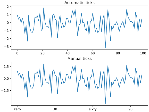

这里的第二幅图使用set_xticks和set_yticks手动设置了刻度线位置和标签。

dates and strings🔗

对于日期，可以使用matplotlib.dates模块来处理日期，例如（详细见Date tick labels）：

from matplotlib.dates import ConciseDateFormatter

fig, ax = plt.subplots(figsize=(5, 2.7), layout='constrained')
dates = np.arange(np.datetime64('2021-11-15'), np.datetime64('2021-12-25'),
                  np.timedelta64(1, 'h'))
data = np.cumsum(np.random.randn(len(dates)))
ax.plot(dates, data)
ax.xaxis.set_major_formatter(ConciseDateFormatter(ax.xaxis.get_major_locator()))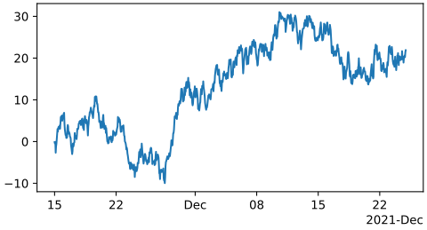

这里dates生成了从2021-11-15到2021-12-25每个小时的日期序列，而data是根据dates生成的随机数据。

对于字符串，我们使用分类绘图（详细见Plotting categorical variables）：

fig, ax = plt.subplots(figsize=(5, 2.7), layout='constrained')
categories = ['turnips', 'rutabaga', 'cucumber', 'pumpkins']

ax.bar(categories, np.random.rand(len(categories)))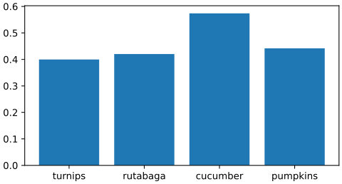

其他轴对象🔗

有些时候可能还需要额外的轴，这时可以使用twinx和twiny添加一副新图（详细见Plots with different scales），或使用secondary_xaxis和secondary_yaxis（详细见Secondary Axis）添加一个新轴：

fig, (ax1, ax3) = plt.subplots(1, 2, figsize=(7, 2.7), layout='constrained')
l1, = ax1.plot(t, s)
ax2 = ax1.twinx()
l2, = ax2.plot(t, range(len(t)), 'C1')
ax2.legend([l1, l2], ['Sine (left)', 'Straight (right)'])

ax3.plot(t, s)
ax3.set_xlabel('Angle [rad]')
ax4 = ax3.secondary_xaxis('top', (np.rad2deg, np.deg2rad))
ax4.set_xlabel('Angle [°]')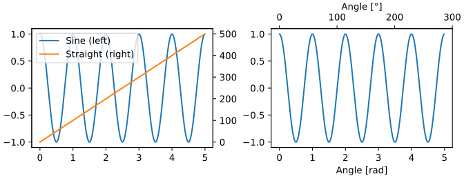

这里的第一幅图使用twiny添加了一个新图，第二幅图使用secondary_xaxis添加了一个新轴。

颜色映射数据🔗

有时希望用颜色来表示第三个维度，在Matplotlib中有很多绘图类型可以做到这一点：

from matplotlib.colors import LogNorm

X, Y = np.meshgrid(np.linspace(-3, 3, 128), np.linspace(-3, 3, 128))
Z = (1 - X/2 + X**5 + Y**3) * np.exp(-X**2 - Y**2)

fig, axs = plt.subplots(2, 2, layout='constrained')
pc = axs[0, 0].pcolormesh(X, Y, Z, vmin=-1, vmax=1, cmap='RdBu_r')
fig.colorbar(pc, ax=axs[0, 0])
axs[0, 0].set_title('pcolormesh()')

co = axs[0, 1].contourf(X, Y, Z, levels=np.linspace(-1.25, 1.25, 11))
fig.colorbar(co, ax=axs[0, 1])
axs[0, 1].set_title('contourf()')

pc = axs[1, 0].imshow(Z**2 * 100, cmap='plasma', norm=LogNorm(vmin=0.01, vmax=100))
fig.colorbar(pc, ax=axs[1, 0], extend='both')
axs[1, 0].set_title('imshow() with LogNorm()')

pc = axs[1, 1].scatter(data1, data2, c=data3, cmap='RdBu_r')
fig.colorbar(pc, ax=axs[1, 1], extend='both')
axs[1, 1].set_title('scatter()')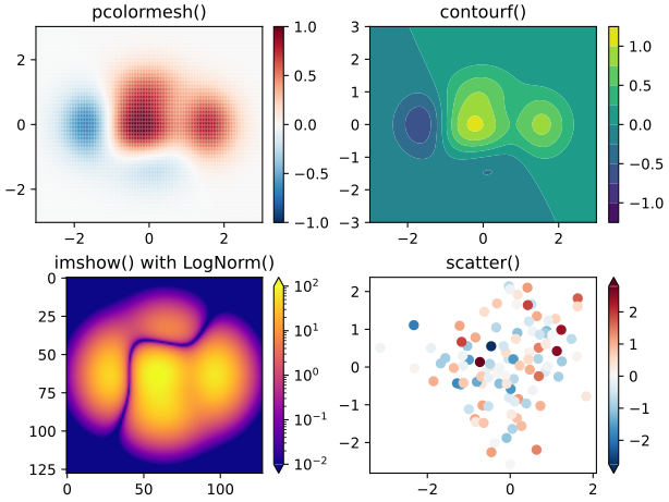

这里分别使用了pcolormesh、contourf、imshow和scatter四种方法。

Colormaps🔗

这些都是ScalarMappableArtists，都可以将vmin和vmax之间的线性映射设置为cmap指定的Colormaps（Colormaps见Choosing Colormaps in Matplotlib）。

Normalization🔗

有时我们希望数据到颜色图的映射是非线性的，这个时候要提供norm参数而不是vmin和vmax参数（详细见Colormap normalization）。

Colorbar🔗

添加一个Colorbar用于查看颜色与数据的关系，用extend参数控制Colorbar的外观，用shrink和aspect参数控制大小。关于Colorbar的放置位置，见Placing colorbars。

使用多个Figures和Axes🔗

可以多次调用plt.figure()或plt.subplots()来创建多个Figure.

添加多个Axes有很多方法，可以用plt.subplots()，要添加更复杂的可以使用subplot_mosaic（详细见Arranging multiple Axes in a Figure和Complex and semantic figure composition (subplot_mosaic)）：

fig, axd = plt.subplot_mosaic([['upleft', 'right'],
                               ['lowleft', 'right']], layout='constrained')
axd['upleft'].set_title('upleft')
axd['lowleft'].set_title('lowleft')
axd['right'].set_title('right')